Solubility – Ideal Solubility & Solubility Models
Solubility is defined as the property of a solid, liquid, or gaseous chemical substance, called the solute, to dissolve in a solid, liquid, or gaseous solvent and form a homogeneous solution of the solute in the solvent – note that this refers to a non-reactive interaction1. The solubility of a substance depends on the solvent as well as temperature and pressure. It is a balance of inter-molecular forces between the solvent and solute, and the entropy change that accompanies the solvation. In pharmaceutical development, solubility of an active pharmaceutical ingredient (API) is routinely measured in a variety of organic solvents, aqueous solutions, and polymers as part of a pre-formulation program. These data are used to guide formulation development and analytical method development. This technical brief will focus on solubility of APIs in solvents, polymers, and bio-membranes. What follows are practical approaches to thinking through solubility issues, including how to efficiently identify the most likely formulation possibilities.
Ideal Solubility
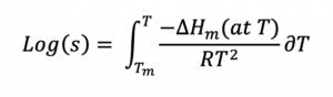
A logical starting point for approaching formulation development is “ideal solubility”, defined as the solubility of a solute in the perfect solvent for which there is no energy penalty associated with the dissolution process2. This definition of ideal doesn’t cover cases where there are specific chemical reactions (i.e., acid-base) or ionic effects (in water) associated with dissolution. The ideal solubility depends only on the energy penalty needed to break the crystalline structure of the API – the API has to “melt” before it can dissolve. If the enthalpy of fusion, the melting point, and heat capacities are known, the ideal solubility can be calculated exactly by:
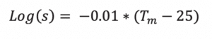
If just the melting point is known, the Yalkowsky approximation is surprisingly useful in predicting the (mole fraction) solubility at 25°C 2:
From a practical perspective, estimating the ideal solubility is worthwhile as it will prompt the formulator to investigate alternate formulation methods rather than spend time attempting to develop a solubilizing formulation approach when the ideal solubility is too low for the intended application. One can’t fight the laws of thermodynamics.
When substances are mixed, deviations from ideality begin to occur. These deviations are caused from the various interactions between the mixed species and are captured in the decreased activities of each substance. In some cases, such as binary systems with simple interactions, it may not be too difficult to obtain activities and activity coefficients. In practice, formulations will likely have multiple materials such as solubilizers, surfactants, plasticizers, and other types of excipients as well as one or more API, making measuring and use increasingly complex and time consuming.
Solubility Models
Over the past few decades, multiple models have been developed to make solubility predictions more practical. The simpler models such as those based on octanol/water partition coefficient (Log P) or polar/non-polar interactions provide a starting point but are limited in the sense that two substances, each with a high Log P, or two substances that are non-polar, may not be miscible with each other. The more complex models include various quantitative structure activity relationships, quantum mechanical and thermodynamic tools such as COSMOtherm, and others such as those based on Abraham parameters or Non-random Two-Liquid Segment Activity Coefficients3-5.
Hansen Solubility Parameters
The model that will be the focus of this technical brief is Hansen Solubility Parameters (HSP) 6,7. HSP are relatively simple to use while maintaining a degree of accuracy needed for practical use. Not surprisingly, such simplicity comes with limitations. However, they provide a lot of guidance for real-world, less-than-ideal formulations, where other tools are not easily applied. Additionally, the same HSP approach applies to polymers, nanoparticles, excipients, and bio-membranes such as skin. This allows rational decisions to be made about blends of polymers and excipients that optimize the solubility behavior.
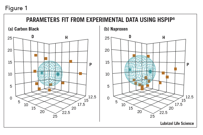
At the heart of HSP is the concept that “like dissolves like”. Each solvent, API, polymer, nanoparticle, bio-membrane, etc. can be assigned the three HSP – D, P, H. Their “likeness” is calculated by a simple 3-D distance calculation and can be visualized graphically using the computer program HSPIP6. In Figure 1, graphical depictions of carbon black (1a) and naproxen (1b) are shown – their HSP are in the center of their respective spheres. In the figure, D refers to the D, P refers to P, and H refers to H. The three parameters are intuitive. D represents the dispersion (van der Waals) property of a molecule. This represents the general polarizable electrons in each molecule and is never zero – all molecules attract each other via dispersion forces. The P value represents the polar attribute of a molecule and correlates well with the dipole moment. H represents hydrogen bonding, both donor (such as chloroform) and acceptor (such as acetone) as well as traditional hydrogen bonding groups such as –OH.
If the HSP of an API (1) and a polymer (2) are known, then the HSP distance between them is:
![]()
The smaller the distance, the more alike the API and the polymer are and therefore the higher the solubility of the API, ease of dispersion, Fickian diffusion out of the polymer, etc.
To relate an API to any other material, the HSP of that API must be known. The methods of determining the parameters can be experimental or predicative with an agreement between both being desired.
The three parameters are defined as:
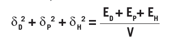
where V is the molar volume and Ei is the cohesion energy of the i type interactions. The left side adds up to the square of the Hildebrand solubility parameters from which Hansen’s parameters are based. The total cohesion energy can be determined by the energy of vaporization, but segmenting it based on different interactions is difficult and therefore various approaches have been developed to arrive at the HSP.
The most rigorous is by statistical thermodynamic calculations and is more involved than can be described here7. Several group contribution methods exist in which the molecule is broken down into many smaller sections. These sections each have known parameters that can be combined to give an overall set of HSP for the molecule in question. Experimental methods can also be used where the solubility of the substance is measured in a variety of solvents and the data are fit on the basis that “like dissolves like.” The molecule’s parameters will be most similar to the parameters of the solvents it most readily dissolves into.
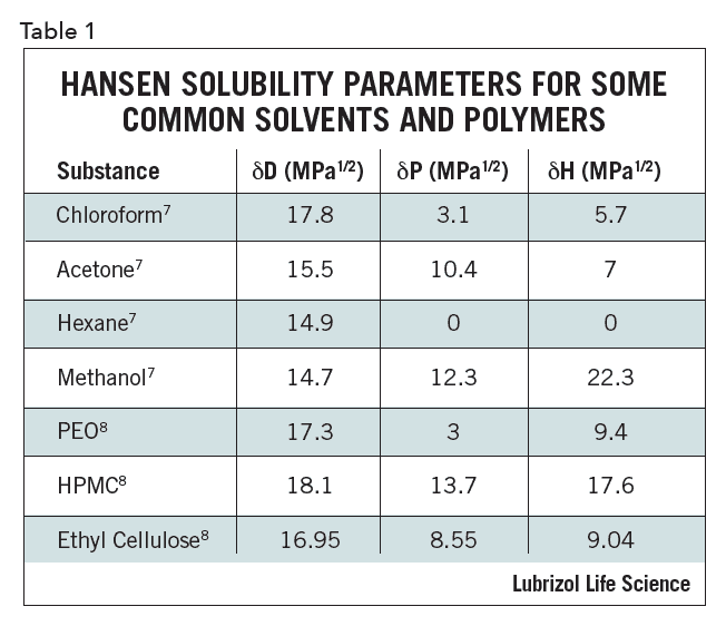
Utilizing tools such as HSP impacts the pharmaceutical formulation process as early as the pre-formulation stage by reducing the resources and consumables spent in the lab and providing a logical approach to considering which materials may be best suited for a particular formulation. One example is solvent or excipient replacement. The HSP of a mixture of two solvents is the weighted average of their volume percent. Even more important is two solvents that individually have a large HSP distance from an API can be close as a mixture: in other words, two poorly solubilizing solvents can, when combined, effectively dissolve an API. If it is known that a hazardous solvent can easily solubilize an API, then two safe materials can be found that have similar HSP as the solvent when combined. This fact can be exploited to optimize compatibility/solubility, combining solvents or excipients in novel ways. Representative HSP for select solvents and polymers are given in Table 1.
 The HSP of skin can be estimated and formulations can be rationally optimized either to the API (getting a small HSP distance to ensure maximum API solubility) or the skin (to get the maximum amount of formulation into the skin) or somewhere in between if you wish to balance API loading and delivery onto or into the skin. Along the same line, if the formulation’s HSP are optimized to interact with the skin, the API will likely be at higher concentrations near the formulation-skin interface.
HSP also provide a way to analyze or design surfactants. Since the two ends of surfactants tend to have different solubilizing capabilities, each end has its own set of parameters. This can be used to choose a hydrophobic tail with HSP similar to that of an API. When the system is placed in an aqueous media, micelles will form with the API contained inside.
Conclusion
Solubility of an API helps shape the formulation approach. Poorly soluble drugs require more creative approaches to deliver the API to the targeted site compared to drugs that are easily solubilized. Predictive tools such as ideal solubility and Hansen solubility parameters can provide insight into many problems that will be encountered throughout formulation development. These tools can be useful in suggesting formulation approaches, which may increase development efficacy and shorten the development cycle.
References
- http://en.wikipedia.org/wiki/Solubility
- H. Yalkowsky and M. Wu, “Estimation of the Ideal Solubility (Crystal–Liquid Fugacity Ratio) of Organic Compounds”, J. Pharm. Sci., 99(3), March 2010, pp 1100-1106.
- cosmologic.de
- H. Abraham, R.E. Smith, R. Luchtefeld, A.J. Boorem, R. Luo, and W.E. Acree Jr., “Prediction of Solubility of Drugs and Other Compounds in Organic Solvents”, J. Pharm. Sci., 99(3), March 2010, pp 1500-1515.
- -C. Chen and Y. Song, “Solubility Modeling with a Non-random Two-Liquid Segment Activity Coefficient Model’, Ind. Eng. Chem. Res., 43, 2004, pp 8354-8362.
- HSPiP, hansen-solubility.com
- M. Hansen, “Hansen Solubility Parameters: a User’s Handbook.” Boca Raton: CRC, 2007.
- Chan, K. Coppens, V. He, P. Jog, and P. Larsen, “Solubility Parameters as a Tool to Predict API Morphology in Hot Melt Extrusion (HME) Formulations Containing Ethylcellulose, Hypromellose, and Polyethylene Oxide.” October 2006. The Dow Chemical Company.