Considerations in Particle Sizing – Part 1: Classification of the Various Sizing Techniques

Choosing the correct particle size (PS) analyzer for a given sizing need can be a challenging process. There are a host of commercially available instruments: image analyzers, single particle counters, fractionation devices, ensemble averaging devices, and single-moment (average) devices, plus the variations within each technique. Marketing hype surrounding specifications and performance further confounds the decision-making process. The idea that one instrument will suit every particle sizing need is not accurate.

Particle size analysis techniques are often misused because of a lack of understanding of their underlying principles and confusion arising from the marketing hype. The theoretical basis for the many “classical” and “modern” techniques^1-6 has been extensively reviewed. Additionally, manufacturer’s literature can also be a good resource^{7, 8} and an excellent practical guide has been published by NIST⁹. A study of methods used for PS analysis of dry active pharmaceutical ingredients (API) powders is available¹⁰ and a recent paper addresses the use of laser diffraction to size sub-micron API particles and highlights the problems involved¹¹.

This technical brief is focused on the sizing of particles in liquids and is based on the authors’ many years of collective experience with the various methods of analysis. The aim is to provide a pathway through the decision-making process by means of asking and answering three questions:

1. How do I classify the various techniques?
2. How do I set specifications (either quantitative or qualitative)?
3. Which technique(s) have the best chance of solving my problems?

CLASSIFICATION OF PARTICLE SIZING TECHNIQUES

All techniques can be classified in any of the following five ways: (i) size range, (ii) degree of separation (i.e., fractionation), imaging vs. non-imaging methods, (iv) weighting: intensity, volume, surface, number and (v) information content.

Through a review of these common ways to classify the available techniques it should be possible for the user to reduce the number of choices to one or two.

Size Range

Eighteen commercially available particle sizing techniques are shown in Figure 1 together with their approximate size ranges; the following are points to consider:

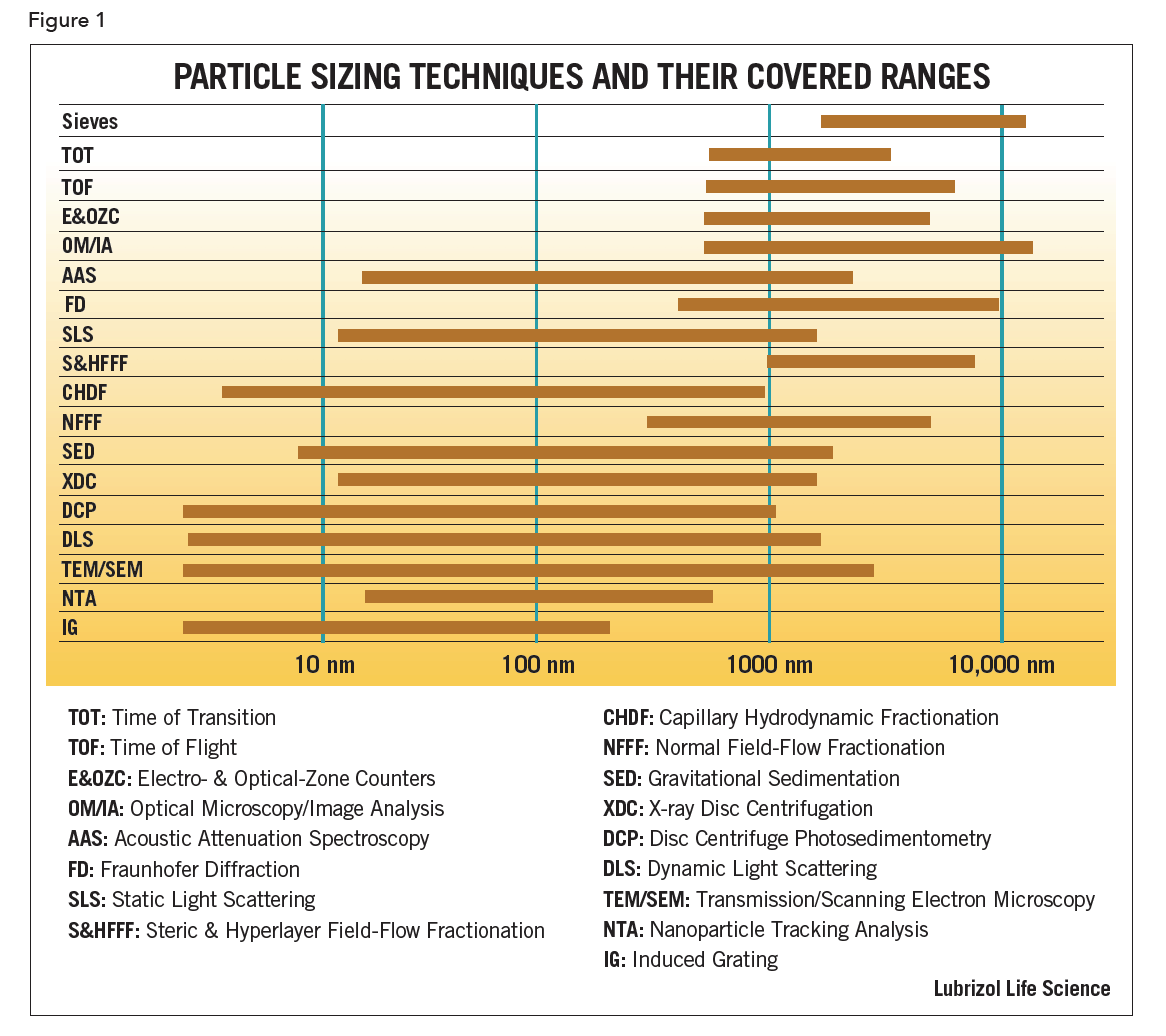
First, there are theoretical limitations either in the assumptions or the equations used to calculate the results. For example, sedimentation is limited at its upper end by turbulence and at the low end by diffusion. Both density and size will play a role in the choice between sedimentation and centrifugation methods. Diffraction is limited to sizes much larger than the wavelength of the light source used. For particles larger than 1 µm, the classical Fraunhofer Diffusion (FD) pattern is independent of the refractive index (RI) of the material. For smaller particles, the scattering pattern depends significantly on the RI.

Second, there are limitations associated with the implementation. For example, to ensure a good dynamic response, the detectors in diffraction devices are located such that the raw class sizes are logarithmically spaced. This may mean that the last class size covers half the total size range.

Third, there are limiting cases that have become, incorrectly, generalized to cover all types of samples. Dynamic light scattering (DLS) is a versatile technique for particles which remain suspended. Even very large particles (ca 1 µm) of materials of low density, such as polystyrene latex (µ=1.01) can stay suspended in water long enough to make useful measurements but, for high density materials such as ZnO (µ=5.6), the upper size range is restricted.

Finally, there are limitations when different techniques are spliced together to extend the operational size range of an instrument. While possible in principle, it is difficult to achieve in practice without producing artifacts. Usually each sub-range will require a change in something: a lens, an aperture, a speed of rotation, etc., inducing artifacts that can be mistaken as real. Smoothing can be applied to the data to reduce, or hide, artifacts but this can then result in a loss of resolution. Different techniques use different weightings and are subject to theoretical limitations, especially at their extremes – yet it is at the extremes where they are spliced together.

To select a particle sizing technique, the user should determine the size range of interest, then narrow the search to those instruments covering that range. Never use a technique at the extremes of its size range capability. Special care must be taken during both the sampling process and sample preparation. Although it can be easy to believe that an instrument with the widest claimed-for range of application is the most effective, it may not be the optimum choice.

Degree of Separation

There are three categories: (i) single particle counting, (ii) fractionation and (iii) ensemble averaging. Imagine a distribution of separate, perfect spheres of different sizes. Then add a ruler for measuring each diameter. This describes single particle counting (SPC) using image analysis. If the number of particles of different sizes is sufficiently large, such a method is perfect: it results in the highest degree of separation – the ultimate resolution is achieved. SPC is the best choice when absolute concentration as a function of size is required. But even SPC devices can have problems. With imaging techniques, sample preparation can lead to artificial aggregation or agglomeration. The number of particles per image has to be limited in order to achieve full separation. Thus, for reasonable statistics, many images need to be analyzed. Particles not entirely within a single frame need to be subjectively discounted; close attention must be also paid to focusing and shadowing effects. Also, image analysis requires calibration. For irregular shape particles, complex algorithms have to be applied and assumptions made.

For non-imaging SPC such as zone counters, time-of-flight and time- of-transition instruments statistical problems are a major concern. With zone counters, clogging of orifices do occur and corrections for coincidence counting must be applied at the low end of the size range; calibration is also necessary. The next level down in degree of separation and resolution is an instrument that fractionates according to size (and, perhaps, another parameter such as density) prior to size determination. The classic example is the sieve. Modern fractionation devices include sedimentation, column-based separation and the various field-flow fractionation techniques. As a class, these techniques tend to be relatively slow but provide reasonable separation and resolution to satisfy most sizing requirements.

Ensemble averaging techniques include FD and all forms of light scattering (dynamic (DLS), static (SLS), etc.). In general, the resolution is low since the particles are neither counted nor physically separated. In these devices the raw data is mathematically deconvoluted to produce size distribution information. Information is lost since the signals are often complicated non-linear functions of size. Unless fractions are narrow and more than 2:1 apart in size, accurate bi-modal distributions are not possible. As a class, ensemble averaging PS analyzers are fast, easily automated and can in principle be put online.

Despite lack of resolution, two such techniques, namely DLS and FD (with or without high-angle scattering), are among the most popular of all particle sizing techniques. The reasons are speed of measurement, versatility and the fact that for many sizing applications only modest resolution is often all that is required.

In choosing a suitable particle sizing technique, the user should ask what degree of separation is sufficient. For example, in Quality Control, a broad, low-resolution “snap-shot” of size distribution may be all that is needed.

Imaging vs. Non-imaging Methods

Imaging techniques include optical and electron microscopy, video, holography and photography. Image analyzers suffer from coincidence effects and tend to be expensive. Manual analysis is subjective, slow and labor intensive. When automated to increase efficiency, coincidence effects are difficult to recognize.

With few exceptions, when shape information (such as aspect ratios, jaggedness of abrasives, fractal nature of aggregates, etc.) is required, there is no substitute for an image analyzer. Image analyzers are also useful for quantifying texture, color and composition. In special cases, multi-angle light scattering can yield an average fractal number.

All non-imaging techniques yield equivalent spherical diameters (ESD), the diameter of a sphere that would give the same result as the actual particle. Thus, different techniques may yield a different ESD for the same particle. Nevertheless, these differences are valuable since they can reveal in- formation on the shape, structure or texture of the particle.

Consider also the following example of a bimodal, differential, volume-weighted distribution determined using a non-imaging ensemble averaging device (Figure 2).

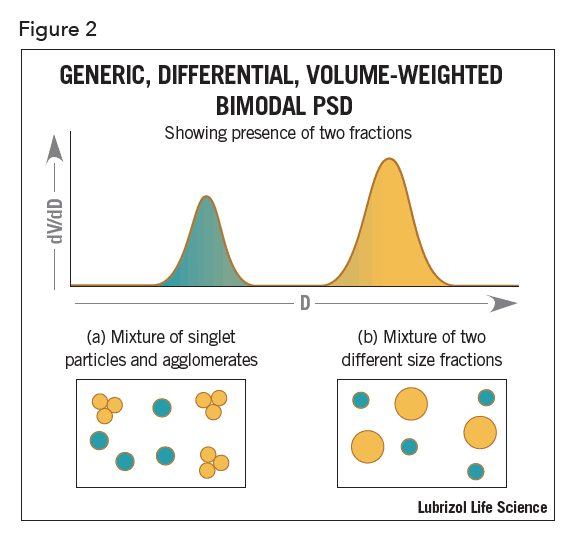There is no way to determine if the modes arise from singlet particles plus a second fraction comprising agglomerates of those particles (Figure 2a) or a simple mixture of two different fractions of singlet particles each of a different size (Figure 2b). Both particle size distributions would result in a bimodal as shown, making it difficult to distinguish. However, image analysis can easily distinguish between a mixture of two separate modes and agglomerates.

Weighting: Intensity, Volume, Surface Area, Number

Different techniques will weigh the raw data differently. For example, sieve data, assuming all particles have the same density, is mass- or volume-weighted, whereas SPC gives number-weighted data. Volume and number weightings vary as size raised to the 3rd- and zero-order, respectively. Intensity-weighting is not so simple. For DLS measurement of very small particles, the intensity of the light scattered particles is weighted by the 6th power of the diameter. When measuring very large particles using FD, the intensity is weighted by the square of the diameter

If possible, a technique should be chosen whose fundamental weighting is closest to that which is needed, or used, in practice. In pharmaceutical applications, either volume- or number-weighted data is the most useful. Volume-weighted data is more appropriate for pharmaceutical products administered via intravenous injection, so as to be able to detect a few large particles in a sea of smaller ones. Number-weighted data is useful if you are interested in tracking the specific surface area of a sparingly water-soluble API formulation intended for oral administration. The specific surface area correlates directly to the rate of dissolution of the API.

Although equations are available for converting one type of weighting to another, the results calculated this way are often erroneous, especially in the case of intensity-weighting in part because of the assumptions that need to be made. Also, algebraic transformations using powers of diameter mask over the more important issue of signal-to-noise-ratio. For example, a small artifact at low particle size, when transformed from intensity- to number-weighting, suddenly becomes completely dominant. When two different techniques are concatenated in the hopes of covering a much larger range in particle size, a difficulty arises because of the way in which each weights the raw data. In addition, other practical problems in combining raw data arise from sampling, changes in resolution and boundary matching. Inevitably these problems often outweigh the advantages. An instrument that covers a smaller, reasonable size range correctly will always be superior to one that claims zero to infinity.

Part 2 will cover the fifth way to classify a particle sizer and then conclude by providing guidance for specifying a particle size analyzer.

REFERENCES

1. D. Stockham and E.G. Fochtman (eds), Particle Size Analysis, Ann Arbor Science Publishers, Ann Arbor, 977
2. Kaye, Direct Characterization of Fine Particles, Wiley-Interscience, London, 1981
3. Barth (ed), Modern Methods of Particle Size Analysis, Wiley-Inter- science, New York, 1984
4. Allen, Particle Size Measurement, 4th Edition, Chapman & Hall, New York, 1990
5. G. Stanley-Wood and R.W. Lines (eds), Particle Size Analysis, Royal Society of Chemistry, London, 1992
6. Provder (ed), Particle Size Distribution: Assessment and Characterization, ACS Symposium Series 332 (1987), 472 (1991), 693 (1998) and 88 (2004), American Chemical Society, Washington, DC.
7. CPS Instruments Inc. Comparison of Particle Sizing Methods
8. Micromeritics Instruments Inc., Interpretation of Particle Size Reported by Different Analytical Techniques
9. Jillavenkatesa, S.J. Dapkunas and L-S. H. Lum, Particle Size Characterization, NIST Special Publication 960-1, 2001
10. M. Etzler and M.S. Sanderson, J. Particle and Particle Systems Characterization 2 217 (1995)
11. M. Keck and R.H. Muller Int. Journal Pharmaceutics 355 150 (2008)